Velocity types – Methods of defining velocity profiles

This method assigns a constant (not time variant) interval velocity to the velocity layer.

By entering a velocity value in the ‘V’ column on the Velocity Model form you determine that this value should be used everywhere in that layer. To use laterally varying interval velocities, you need to create a 2D grid property of type ‘Velocity’ for the base surface time horizon (see Using laterally varying V0 and k). If present, it will be shown as a selectable item in the drop-down list of the ‘V’ column.

Interval velocity is the average velocity over a given interval.

This velocity profile type is probably the method most commonly used for stratified velocity fields. It assumes that a linear relation exists between depth (absolute depth, or below a compaction reference surface) and interval velocity, reflecting compaction behavior. This means that when you depth convert time objects, this generates a less 'blocky' velocity profile than when you use constant interval velocities.

The input parameters ‘V’ and ‘k’ are usually derived by regression of interval velocities against depth. In deciding on an appropriate layer breakdown it is worth considering that more layers do not mean more accurate depth conversion: thin layers can cause erroneous velocity extrapolation effects.

By entering values in the ‘V’ (in this case ‘V₀’) and ‘k’ columns on the Velocity Model form, you determine that these parameters should be used everywhere. To use laterally varying parameters you need to create 2D grid properties of type ‘Velocity’ or ‘k’ for the base surface time horizon (see Using laterally varying V0 and k). If present, they will show as selectable items in the drop-down lists of the ‘V’ and ‘k’ columns.

Instantaneous velocity (Vinst) is the velocity at a specific point at depth z within a given interval. The linear function describes how Vinst varies over the interval as z changes in relation to gradient k. Vinst can also be described as the rate of change of depth with time over a given interval. Using this function, instantaneous velocity at a specific depth point within the interval can be estimated.

This method can capture large-scale vertical trends in instantaneous velocity in a simple function. It is used in sequences where large-scale vertical velocity trends occur related to lithology variations and compaction effects are subordinate (e.g. with large-scale shallowing upward cycles from shale to carbonate). Accordingly, this method is usually referenced to the upper velocity layer (TVD value of base of upper velocity layer or base surface of the upper velocity layer).

The input parameters ‘V’ and ‘k’ are usually derived by regression of instantaneous velocities (e.g. form integrated sonic logs) against depth. V₀ is usually fixed while k may be varied as a function of interval thickness.

By entering values in the ‘V’ (in this case ‘V₀’) and ‘k’ columns on the Velocity Model form you determine that these parameters should be used everywhere. To use laterally varying parameters you need to create 2D grid properties of type ‘Velocity’ or ‘k’ for the base surface time horizon (see Using laterally varying V0 and k). If available, they will show as selectable items in the drop-down lists of the ‘V’ and ‘k’ columns.

Average velocity describes the velocity gradient from ground level or seafloor (mudline) to base interval, and can only be used (in the application) for the overburden or as a second layer below a water layer.

V₀k functions predicting average velocity are used in monotonous compacting clastic sediments, i.e. where lithologies with exotic velocities are absent or confined to thin intervals with little variation in thickness. Under these circumstances it is appropriate to use a single velocity layer from surface to deepest target or top overpressures.

The input parameters ‘V’ and ‘k’ are derived by regression of average velocities against depth, e.g. analyzing checkshot/VSP data.

By entering values in the ‘V’ (in this case ‘V₀’) and ‘k’ columns on the Velocity Model form you determine that these parameters should be used everywhere. To use laterally varying parameters you need to create 2D grid properties of type 'Velocity' or ‘k’ for the base surface time horizon (see Using laterally varying V0 and k). If available, they will show as selectable items in the drop-down lists of the ‘V’ and ‘k’ columns.

     click to enlarge

This method is applicable under the same conditions as the V₀kz method above but has two advantages over it. Firstly, actual checkshot/VSP data covering large depth intervals frequently show a more linear behavior in V_avg-time graphs than in V_avg-depth graphs. Secondly, the V₀ and k parameters in V_avg-time systems correspond directly to the A and B terms in second order t-d regressions forced through 0.

The input parameters ‘V’ and ‘k’ can be derived directly by regression of average velocities against 2-way time or indirectly from the A and B terms of second order functions in time-depth, e.g., analyzing checkshot/VSP data.

By entering values in the ‘V’ (in this case ‘V₀’) and ‘k’ columns on the Velocity Model form you determine that these parameters should be used everywhere. To use laterally varying parameters you need to create 2D grid properties of type 'Velocity’ or ‘k’ for the base interval time horizon (see Using laterally varying V0 and k). If available, they will show as selectable items in the drop-down lists of the ‘V’ and ‘k’ columns.

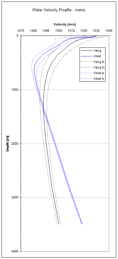
If you are dealing with an offshore project, then consider using the ‘Water Velocity Profile Avg’ method, which makes use of water velocity lookup tables. Water velocity is primarily a function of depth, temperature, and salinity. The implementation in the application is based on velocities derived with the McKenzie (1981) function from temperature and salinity data collected globally in marine continental slope settings by the US Navy.

When using the option ‘Water Velocity Profile Avg’ you can scale the lookup of velocities between minimum and maximum by entering values between -1 and 1 in the table column 'Water Velocity Profile Factor', where:

Based on the value you enter, the table values are weighted. For example, when you enter 0.5, the average of the values of Vavg and Vmax will be taken.

This method is an automated implementation of the 'V_int from user input' with laterally varying interval velocity. For pairs of time horizons and depth markers, time values are extracted from horizons at the location of well markers. Interval velocities are then calculated and stored with the respective well marker, and interpolated between well markers using a user-defined method, to obtain complete area coverage.

It is appropriate for cases with either little structural relief, and thus little difference in compaction state, and cases with comprehensive well control, i.e. where forward modeling of velocity is not necessary.

Precondition for using this method is that markers and horizons represent the same geological events, i.e. the need to have identical names in the JewelExplorer. Calculated interval velocities are stored as velocity properties with the respective markers and can be QC’ed by selecting this marker property in the JewelExplorer.

If you want to use other interpolation methods or parameters other than those built into the automated option then you can do so with the Property Calculator. For more information, see Using the Property Calculator to interpolate velocities and Creating your own depth conversion methods with the Property Calculator.